Quickstart

This guide shows the three ways to define a sampling grid in healpix-plot, from the simplest dict shorthand to a pixel-aligned affine grid.

Setup

import numpy as np
import matplotlib.pyplot as plt
import cartopy.crs as ccrs
import healpix_plot

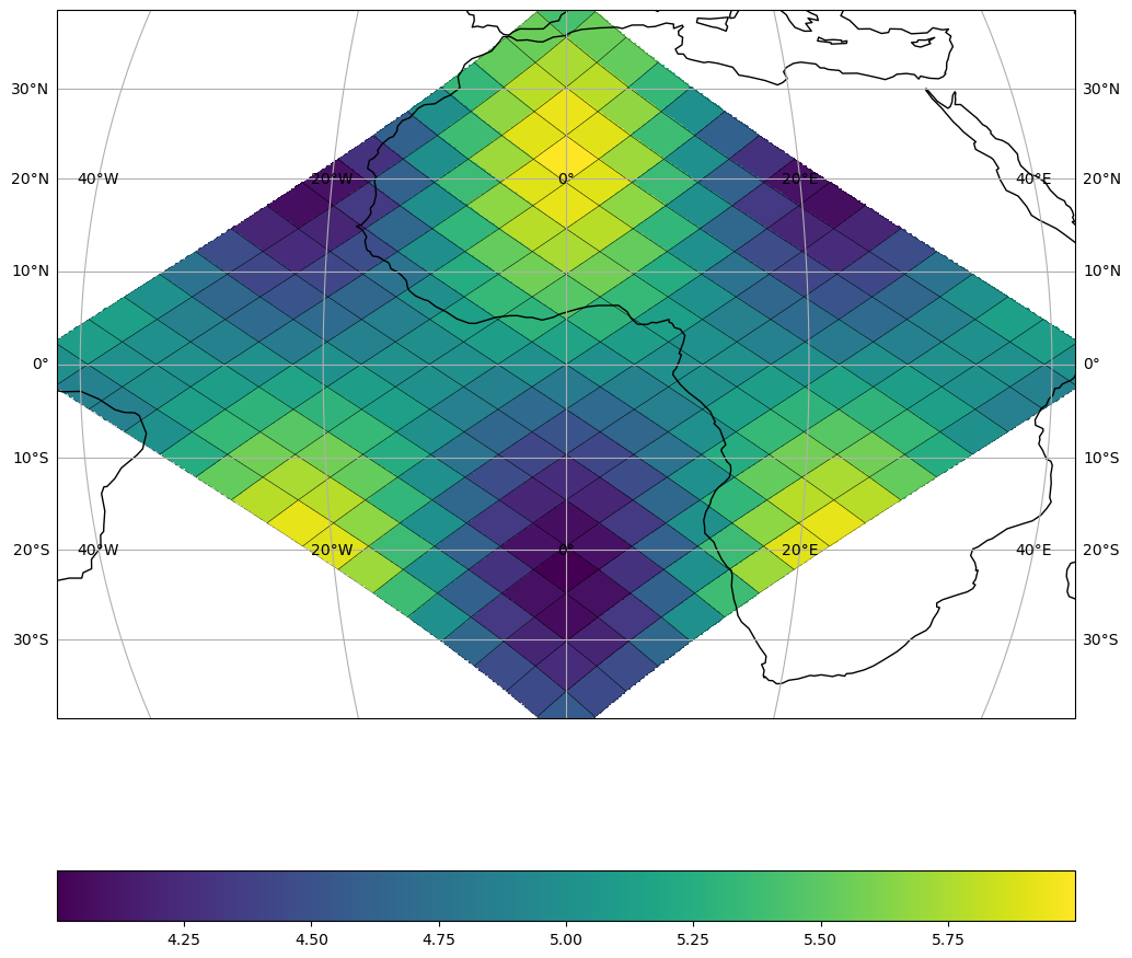
1 — Dict shorthand

The simplest way: pass {"shape": N} and the spatial extent is inferred automatically from the cell IDs.

In real workflows your cell_ids and data come from a file (NetCDF, Zarr, …). Here we use a synthetic wave pattern.

healpix_grid = healpix_plot.HealpixGrid(
    level=3, indexing_scheme="nested", ellipsoid="WGS84"
)

cell_ids = np.arange(
    4 * 4**healpix_grid.level, 5 * 4**healpix_grid.level, dtype="uint64"
)

lon, lat = healpix_grid.operations.healpix_to_lonlat(
    cell_ids, **healpix_grid.as_keyword_params()
)
data = np.cos(8 * np.deg2rad(lon)) * np.sin(4 * np.deg2rad(lat))

print(f"level: {healpix_grid.level}, n_cells: {cell_ids.size}")
print(f"data range: [{data.min():.2f}, {data.max():.2f}]")

level: 3, n_cells: 64
data range: [-0.99, 0.99]

fig, ax = plt.subplots(
    1, 1, subplot_kw={"projection": ccrs.Mollweide()}, figsize=(12, 12)
)

mappable = healpix_plot.plot(
    cell_ids, data, healpix_grid=healpix_grid, sampling_grid={"shape": 512}, ax=ax
)

fig.colorbar(mappable, orientation="horizontal")
ax = mappable.figure.axes[0]

ax.coastlines()
ax.gridlines(draw_labels="x")
ax.gridlines(draw_labels="y")

plt.show()

/home/runner/work/healpix-plot/healpix-plot/.pixi/envs/docs/lib/python3.13/site-packages/cartopy/io/__init__.py:242: DownloadWarning: Downloading: https://naturalearth.s3.amazonaws.com/110m_physical/ne_110m_coastline.zip
  warnings.warn(f'Downloading: {url}', DownloadWarning)

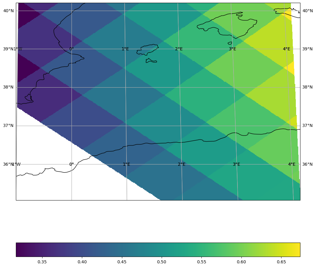
2 — ParametrizedSamplingGrid.from_bbox — fixed region

Use from_bbox when you want to pin the output to a fixed geographic extent, regardless of the data coverage. Useful for regional maps, comparisons, or animations.

Here we zoom in on the western Mediterranean.

from healpix_plot import SamplingGrid
from healpix_plot.sampling_grid import ParametrizedSamplingGrid

# Use WGS84 — the standard geodetic ellipsoid for Earth observation
healpix_grid = healpix_plot.HealpixGrid(
    level=6, indexing_scheme="nested", ellipsoid="WGS84"
)

grid = ParametrizedSamplingGrid.from_bbox(
    bbox=(-20, 35.0, 20, 40.0),  # (xmin, ymin, xmax, ymax) in degrees
    shape=512,
)

cell_ids = np.arange(
    4 * 4**healpix_grid.level, 5 * 4**healpix_grid.level, dtype="uint64"
)


lon, lat = healpix_grid.operations.healpix_to_lonlat(
    cell_ids, **healpix_grid.as_keyword_params()
)
data = np.cos(8 * np.deg2rad(lon)) * np.sin(4 * np.deg2rad(lat))

fig, axes = plt.subplots(
    1, 1, subplot_kw={"projection": ccrs.PlateCarree()}, figsize=(12, 12)
)

mappable = healpix_plot.plot(
    cell_ids, data, healpix_grid=healpix_grid, sampling_grid=grid, ax=axes
)

fig.colorbar(mappable, orientation="horizontal")
ax = mappable.figure.axes[0]
ax.coastlines()
ax.gridlines(draw_labels="x")
ax.gridlines(draw_labels="y")

<cartopy.mpl.gridliner.Gridliner at 0x7f8494b6f890>

/home/runner/work/healpix-plot/healpix-plot/.pixi/envs/docs/lib/python3.13/site-packages/cartopy/io/__init__.py:242: DownloadWarning: Downloading: https://naturalearth.s3.amazonaws.com/10m_physical/ne_10m_coastline.zip
  warnings.warn(f'Downloading: {url}', DownloadWarning)

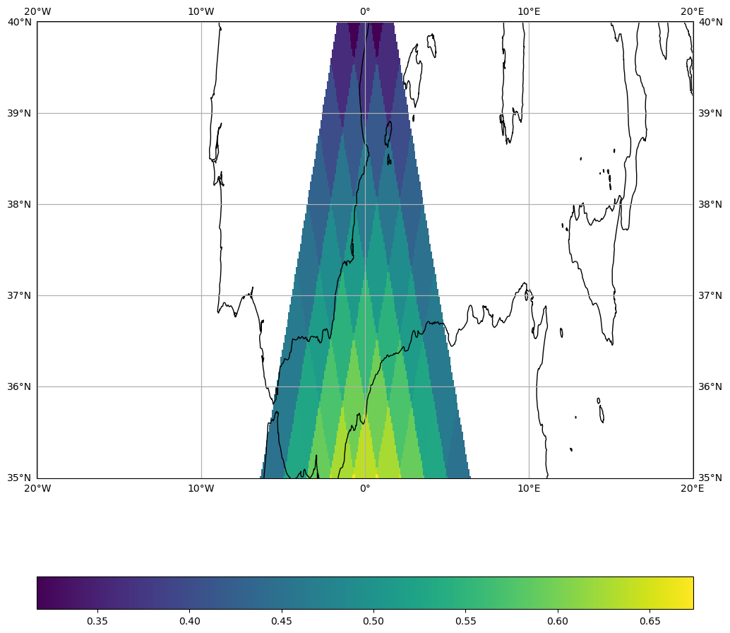
3 — AffineSamplingGrid.from_transform — pixel-aligned grid

Use AffineSamplingGrid when the output pixels must align exactly with a reference raster (e.g. a GeoTIFF). The affine transform maps pixel indices to geographic coordinates: Affine(pixel_width, 0, lon_min, 0, -pixel_height, lat_max).

Here we define a 0.01°/pixel grid (~1 km) over Corsica.

from affine import Affine
from healpix_plot.sampling_grid import AffineSamplingGrid

# Use WGS84 — the standard geodetic ellipsoid for Earth observation
healpix_grid = healpix_plot.HealpixGrid(
    level=6, indexing_scheme="nested", ellipsoid="WGS84"
)

cell_ids = np.arange(
    4 * 4**healpix_grid.level, 5 * 4**healpix_grid.level, dtype="uint64"
)


lon, lat = healpix_grid.operations.healpix_to_lonlat(
    cell_ids, **healpix_grid.as_keyword_params()
)
data = np.cos(8 * np.deg2rad(lon)) * np.sin(4 * np.deg2rad(lat))

transform = Affine(0.01, 0, -1, 0, -0.01, 40)  # 0.01° resolution
grid = AffineSamplingGrid.from_transform(transform, shape=(512, 512))

fig, axes = plt.subplots(
    1, 1, subplot_kw={"projection": ccrs.Mollweide()}, figsize=(12, 12)
)

mappable = healpix_plot.plot(
    cell_ids, data, healpix_grid=healpix_grid, sampling_grid=grid, ax=axes
)

fig.colorbar(mappable, orientation="horizontal")
ax = mappable.figure.axes[0]
ax.coastlines()
ax.gridlines(draw_labels="x")
ax.gridlines(draw_labels="y")

<cartopy.mpl.gridliner.Gridliner at 0x7f8494e27250>

Recipe: overlay true HEALPix boundaries

For sanity checks or presentations you can combine fast raster plots from healpix-plot with boundary polygons from xdggs:

Show code cell source

Hide code cell source

import numpy as np
import healpix_plot
import xdggs
import cartopy.crs as ccrs
import matplotlib.pyplot as plt

# grid
healpix_grid = healpix_plot.HealpixGrid(
    level=4, indexing_scheme="nested", ellipsoid="WGS84"
)

cell_ids = np.arange(
    4 * 4**healpix_grid.level, 5 * 4**healpix_grid.level, dtype="uint64"
)

# example data
lon, lat = healpix_grid.operations.healpix_to_lonlat(
    cell_ids, **healpix_grid.as_keyword_params()
)

data = np.cos(8 * np.deg2rad(lon)) * np.sin(4 * np.deg2rad(lat)) + 5

# polygons of cells
info = xdggs.HealpixInfo(
    level=healpix_grid.level, indexing_scheme=healpix_grid.indexing_scheme
)

polys = info.cell_boundaries(cell_ids)

# figure
fig, ax = plt.subplots(
    1, 1, figsize=(12, 12), subplot_kw={"projection": ccrs.Mollweide()}
)

# plot HEALPix data
mappable = healpix_plot.plot(
    cell_ids, data, healpix_grid=healpix_grid, sampling_grid={"shape": 1024}, ax=ax
)

# colorbar
fig.colorbar(mappable, orientation="horizontal")

# add cell boundaries
ax.add_geometries(polys, crs=ccrs.PlateCarree(), facecolor="none", linewidth=0.2)

ax.coastlines()
ax.gridlines(draw_labels=True)

plt.show()